Today I’d like to share a different way to picture matrices—one which is used not only in mathematics, but also in physics, chemistry, and machine learning. Here’s the basic idea. An ![]() matrix
matrix ![]() with real entries represents a linear map from
with real entries represents a linear map from ![]() . Such a mapping can be pictured as a node with two edges. One edge represents the input space, the other edge represents the output space.
. Such a mapping can be pictured as a node with two edges. One edge represents the input space, the other edge represents the output space.

That’s it!
We can accomplish much with this simple idea. But first, a few words about the picture: To specify an ![]() matrix
matrix ![]() , one must specify all
, one must specify all ![]() entries
entries ![]() . The index
. The index ![]() ranges from 1 to
ranges from 1 to ![]() —the dimension of the output space—and the index
—the dimension of the output space—and the index ![]() ranges from 1 to
ranges from 1 to ![]() —the dimension of the input space. Said differently,
—the dimension of the input space. Said differently, ![]() indexes the number of rows of
indexes the number of rows of ![]() and
and ![]() indexes the number of its columns. These indices can be included in the picture, if we like:
indexes the number of its columns. These indices can be included in the picture, if we like:

This idea generalizes very easily. A matrix is a two-dimensional array of numbers, while an ![]() -dimensional array of numbers is called a tensor of order
-dimensional array of numbers is called a tensor of order ![]() or an
or an ![]() –tensor. Like a matrix, an
–tensor. Like a matrix, an ![]() -tensor can be represented by a node with one edge for each dimension.
-tensor can be represented by a node with one edge for each dimension.
A number, for example, can be thought of as a zero-dimensional array, i.e. a point. It is thus a 0-tensor, which can be drawn as a node with zero edges. Likewise, a vector can be thought of as a one-dimensional array of numbers and hence a 1-tensor. It’s represented by a node with one edge. A matrix is a two-dimensional array and hence 2-tensor. It’s represented by a node with two edges. A 3-tensor is a three-dimensional array and hence a node with three edges, and so on.
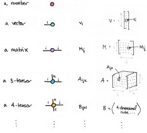
In this graphical notation, familiar things have nice pictures. For example…
Matrix multiplication is tensor contraction.
Multiplying two matrices corresponds to “glueing” their pictures together. This is called tensor contraction.

In the picture above, the edges with matching indices ![]() were the ones that were contracted. This is consistent with the fact that two matrices can be multiplied only when their input/output dimensions match up. You’ll also notice that the resulting picture has two free indices,
were the ones that were contracted. This is consistent with the fact that two matrices can be multiplied only when their input/output dimensions match up. You’ll also notice that the resulting picture has two free indices, ![]() and
and ![]() , which indeed defines a matrix.
, which indeed defines a matrix.
By the way, a key feature of having these pictures is that we don’t have to carry around indices. So let’s not!
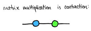
A quick check: A matrix was described as a single node with one edge for each vector space, yet the picture above has two nodes. We still want this to represent a single matrix. And I claim it does! There’s a nice way to see this: simply smoosh the blue and green nodes together.
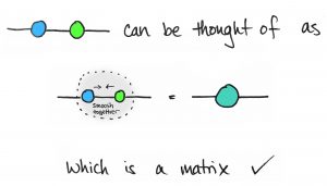
This reminds me of rain trickling down a window: when two raindrops come into contact, they fuse into bigger droplet. That’s matrix-matrix multiplication. A similar picture holds for matrix-vector multiplication: a matrix ![]() multiplied by a vector
multiplied by a vector ![]() results in another vector
results in another vector ![]() , which is a node with one free edge.
, which is a node with one free edge.
More generally, the product of two or more tensors is represented by a cluster of nodes and edges where the contractions occur along edges with matching indices.
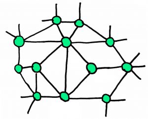
Node shapes can represent different properties.
So far I’ve drawn all the nodes as circles. But this was just a choice. There is no official rule for which shape to use. That means we can be creative! For example, we might want to reserve a circle or other symmetric shape, like a square, for symmetric matrices only.

Then the transpose of a matrix can be represented by reflecting its picture:

So the symmetry of a symmetric matrix is preserved in the diagram!

I also like the idea of drawing isometric embeddings as triangles:
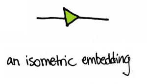
An isometric embedding ![]() is a linear map from a space
is a linear map from a space ![]() into a space
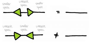
into a space ![]() of larger dimension that preserves the lengths of vectors. Such a map satisfies
of larger dimension that preserves the lengths of vectors. Such a map satisfies ![]() but
but ![]() . In words, you can always embed the small space
. In words, you can always embed the small space ![]() into a larger one, then project back onto
into a larger one, then project back onto ![]() without distorting the vectors in
without distorting the vectors in ![]() . (Not unlike a retraction map in topology.) But you certainly can’t squish all of
. (Not unlike a retraction map in topology.) But you certainly can’t squish all of ![]() onto little
onto little ![]() , then expect to undo the damage after including
, then expect to undo the damage after including ![]() back into
back into ![]() . This large-versus-small feature is hinted at by the triangles. (The base of a triangle is larger than its tip!) And in general, as shown below, identity linear operators are drawn as straight lines:
. This large-versus-small feature is hinted at by the triangles. (The base of a triangle is larger than its tip!) And in general, as shown below, identity linear operators are drawn as straight lines:
Matrix factorizations have nice pictures, too.
With all this talk of matrix multiplication, i.e. matrix composition, let’s not forget about matrix factorization, i.e. matrix decomposition! Every matrix, for example, has a singular value decomposition. This has a nice picture associated to it:

Here, ![]() and
and ![]() are unitary matrices, and hence isometries, and hence triangles. The matrix
are unitary matrices, and hence isometries, and hence triangles. The matrix ![]() is a diagonal matrix, which I like to represent by a diamond. In short, matrix factorization is the decomposition of a single node into multiple nodes; matrix multiplication is the fusion of multiple nodes into a single node.
is a diagonal matrix, which I like to represent by a diamond. In short, matrix factorization is the decomposition of a single node into multiple nodes; matrix multiplication is the fusion of multiple nodes into a single node.
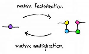
The drawing above illustrates another feature of these diagrams: the spatial position of the nodes doesn’t really matter. I could’ve drawn the yellow, blue, green, and pink nodes in horizontal line, or in a vertical line, or in a zig-zag, or however I wish. The only important thing is that the diagram has two free edges. The product of matrices is another matrix!
Messy proofs reduce to picture proofs.
There’s more we could say about this graphical notation, but I’ll wrap up with another noteworthy feature: proofs can become very simple! Take the trace, for example. The trace of a matrix has a simple picture. It’s defined to be the sum along a common index:
This string-with-a-bead has no free edges. It’s a loop. This is consistent with the fact that the trace is a number. It’s a 0-tensor so it has no free indices. Now here’s a proof that the trace is invariant under cyclic permutations:
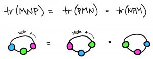
Just slide beads along a necklace. So clean!
What’s in a name?
The diagrams discussed in today’s post, which have their origins in Penrose’s graphical notation, are called tensor network diagrams and/or, perhaps with some minor differences, string diagrams. The “and/or” depends on who you are. That is, the idea to visually represent a map-of-vector-spaces as a node-with-edges is used in the physics/machine learning communities, where they are called tensor network diagrams, and also in the category theory community, where they are called string diagrams. I think this is just a case of different fields using nearly identical notation for different purposes.
Category theorists use string diagrams to prove things. (The diagrams appear in my little booklet on applied category theory, for instance.) What’s more, string diagrams are used to represent most any kind of mapping—not just mappings between vector spaces. Said more formally, string diagrams might arise in a discussion of any monoidal category. For a gentle introduction to these categorical ideas, check out Seven Sketches by Fong and Spivak as well as Picturing Quantum Processes by Coecke and Kissinger.
Some physicists and machine learning researchers, on the other hand, use tensor networks to compute things. A typical situation may go something like this. You have a quantum system. You wish to find the main eigenvector of a special linear operator, called a Hamiltonian. This eigenvector lives in an absurdly large Hilbert space, so you want a technique to find this vector in a compressed kind of way. Enter: tensor networks.
And by “absurdly large,” I do mean ABSURDLY large. If you have an Avogadro’s number’s worth of quantum particles, each of which can occupy just two states, then you need a vector space of dimension ![]() . Now imagine having a linear operator on this space. That’s a matrix with
. Now imagine having a linear operator on this space. That’s a matrix with ![]() entries. That is much much more than the number of atoms in the observable universe. There are only
entries. That is much much more than the number of atoms in the observable universe. There are only ![]() of those! Good luck storing this on a computer. In summary, tensor networks help us deal with a large number of parameters in a principled, tractable way.
of those! Good luck storing this on a computer. In summary, tensor networks help us deal with a large number of parameters in a principled, tractable way.
Tensor networks also have much overlap with graphical models, automata, and more. One vein of current research is identifying and making good use of those overlaps. So there’s a lot to explore here. A few places to start are Miles Stoudenmire’s iTensor library, Roman Orus’s A Practical Introduction to Tensor Networks, Jacob Biamonte’s and Ville Bergholm’s Tensor Networks in a Nutshell, and Google’s TensorNetwork library.
Article by Tai-Danae Bradley* (Research mathematician at Alphabet, Inc)
* This article first appeared on www.math3ma.com and is reproduced here with permission.